Wednesday, November 27, 2013

RSA Key Generation in PyCrypto

In the PyCrypto module for Python the RSA key generator takes a random byte generator to create new keys. The documentation recommends that only a cryptographically secure pseudo random number generator (CSPRNG) be used due to some enhanced security features. The module contains a built-in CSPRNG:
import Crypto
num_bytes = 32
print Crypto.Random.new().read(num_bytes)
Another option however is Microsoft's CryptGenRandom() function. Luckily, in Python, this is easily accessed via the "os" module (os.urandom):
import os
num_bytes = 32
print os.urandom(num_bytes)
Another option for a CSPRNG is Intel's Digital random number generator (DRNG). I didn't even know this existed until recently. If you are fortunate enough to have an Ivy Bridge processor (or later) you will be able to make use of this. Intel has implemented a hardware true CSPRNG in the chip (the generated numbers are truly random). My next project will be to make use of this RNG in Python and PyCrypto.

Thursday, October 10, 2013

Adding Intel's MKL Nonlinear Optimizer to Python as a Module

I was perusing the documentation to Intel's MKL (math kernel library) when I stumbled across their nonlinear optimizer. I wanted to test this optimizer with the levmar routine implemented in a previous post. To do this I have again added it to Python via a module as follows:
#include "Python.h"
#define NPY_NO_DEPRECATED_API NPY_1_7_API_VERSION
#include "arrayobject.h"
#include <iostream>
#include <iomanip>
#include <cmath>
#include <cfloat>
#include "mkl_rci.h"
#include "mkl_types.h"
#include "mkl_service.h"
using namespace std;

struct argstruct {
 double *xval;
 double *yval;
};

double lorentz(double *p, double x) {
 return p[2] / (1.0 + pow((x / p[0] - 1.0), 4) * pow(p[1], 2));
}

void residuals(MKL_INT *m, MKL_INT *n, double *p, double *F, void *data) {
 MKL_INT i=0;
 struct argstruct *bdata;
 double x, y;
 bdata = (struct argstruct *) data;
 for (i=0; i<(*m); i++) {
  x = bdata->xval[i];
  y = bdata->yval[i];
  F[i] = y - lorentz(p, x);
 }
}

static PyObject *mkloptimizer(PyObject *self, PyObject *args) {
 PyArrayObject *xval, *yval, *eps0, *p0;
 argstruct adata;
 double *fvec, *fjac, *p, *eps, r1, r2, res, rs=0.25;
 int count=0;
 MKL_INT iter1 = 100000;
 MKL_INT iter2 = 100000;
 MKL_INT RCI_Request, successful, info[6], iter, st_cr, n, m, i;
 _TRNSP_HANDLE_t handle;

 if (!PyArg_ParseTuple(args, "O!O!O!O!", &PyArray_Type, &xval, &PyArray_Type, &yval, &PyArray_Type, &eps0, &PyArray_Type, &p0)) {
  return NULL;
 }
 m = PyArray_SHAPE(xval)[0];
 n = PyArray_SHAPE(p0)[0];
 adata.xval = (double *) PyArray_DATA(xval);
 adata.yval = (double *) PyArray_DATA(yval);
 eps = (double *) PyArray_DATA(eps0);
 p = (double *) PyArray_DATA(p0);
 // Initialize fvec and fjac arrays
 fvec = new double [m];
 fjac = new double [m*n];
 for (i=0; i<(m*n); i++) {
  if (i<m) {
   fvec[i] = 0.0;
  }
  fjac[i] = 0.0;
 }
 PySys_WriteStdout("Initializing Intel's MKL optimizer ... ");
 if (dtrnlsp_init(&handle, &n, &m, p, eps, &iter1, &iter2, &rs) != TR_SUCCESS) {
  PySys_WriteStdout("FAILED\n");
  MKL_Free_Buffers();
  PyErr_SetString(PyExc_AssertionError, "Initialization error\n");
  return NULL;
 } else {
  PySys_WriteStdout("SUCCESS\n");
 }
 PySys_WriteStdout("Checking optimizer inputs          ... ");
 if (dtrnlsp_check(&handle, &n, &m, fjac, fvec, eps, info) != TR_SUCCESS) {
  PySys_WriteStdout("FAILED\n");
  MKL_Free_Buffers();
  PyErr_SetString(PyExc_AssertionError, "Check optimizer inputs.\n");
  return NULL;
 } else {
  PySys_WriteStdout("SUCCESS\n");
 }
 RCI_Request = 0;
    successful = 0;
 PySys_WriteStdout("\nBegin nonlinear least squares algorithm\n");
 PySys_WriteStdout(" Iter      p[0]      p[1]      p[2]    Residual\n");
 while (successful == 0) {
        if (dtrnlsp_solve(&handle, fvec, fjac, &RCI_Request) != TR_SUCCESS) {
            PyErr_SetString(PyExc_AssertionError,"Error encountered while searching for solution");
            MKL_Free_Buffers ();
            return NULL;
        }
        if (RCI_Request < 0) { 
   PySys_WriteStdout("Algorithm terminated\n");
            successful = 1;
  }
        if (RCI_Request == 1) {
            residuals(&m, &n, p, fvec, (void *) &adata);
   res = 0.0;
   for (i=0; i<m; i++) {
    res += pow(fvec[i],2);
   }
   PySys_WriteStdout("%5d   % 2.4f   % 2.4f   % 2.4f    %2.6f\n", count, p[0], p[1], p[2], sqrt(res));
   count += 1;
        }
        if (RCI_Request == 2) {
            if (djacobix(residuals, &n, &m, fjac, p, eps, (void *) &adata) != TR_SUCCESS) {
                PyErr_SetString(PyExc_AssertionError,"Error encountered in calculation of the Jacobian\n");
                MKL_Free_Buffers();
                return NULL;
            }
        }
    }
 PySys_WriteStdout("\nRetrieving solver's results:\n");
 if (dtrnlsp_get(&handle, &iter, &st_cr, &r1, &r2) != TR_SUCCESS) {
        PyErr_SetString(PyExc_AssertionError,"Error encountered in retrieving results\n");
        MKL_Free_Buffers ();
        return NULL;
    } else {
  PySys_WriteStdout("Number of iterations:\t\t%4d\n", iter);
  PySys_WriteStdout("Initial residual:\t\t%2.18f\n", r1);
  PySys_WriteStdout("Final residual:\t\t%2.18f\n", r2);
  PySys_WriteStdout("Parameter values:\t\t(%2.6f, %2.6f, %2.6f)\n",p[0],p[1],p[2]);
 }


 delete [] fjac;
 delete [] fvec;
 return Py_BuildValue("(d,d,d)", p[0],p[1],p[2]);
}

static PyMethodDef pyMKLoptmethods[] = {
 {"mkloptimizer", mkloptimizer, METH_VARARGS, "Documentation:"},
 {NULL, NULL, 0, NULL}
};

PyMODINIT_FUNC initpyMKLopt(void) {
 Py_InitModule("pyMKLopt", pyMKLoptmethods);
 import_array();
}

Once compiled in Visual Studio you can import the resultant module into Python as follows:
import numpy as np
import pyMKLopt
np.random.seed(22)

DBL_EPSILON = np.spacing(1.0)

def lorentz(p,x):
    return p[2] / (1.0 + (x / p[0] - 1.0)**4 * p[1]**2)
   
p = np.array([0.5, 0.25, 1.0], dtype=np.double)
x = np.linspace(-1.5, 2.5, num=30, endpoint=True)
noisyy = lorentz(p,x) + (np.random.randn(30) * 0.05)
p0 = np.array([1.0, 1.0, 1.0], dtype=np.double) #Initial guess


eps = np.array([1e-8, 1e-20, DBL_EPSILON, 1e-20, 1e-20, DBL_EPSILON], dtype=np.double)
solution = pyMKLopt.mkloptimizer(x, noisyy, eps, p0)
print '\n\n',solution

The output of this script (displayed in the console) is:
Initializing Intel's MKL optimizer ... SUCCESS
Checking optimizer inputs          ... SUCCESS

Begin nonlinear least squares algorithm
 Iter      p[0]      p[1]      p[2]    Residual
    0    1.0000    1.0000    1.0000    1.521464
    1    0.5798   -0.1432    0.8439    1.151126
    2    0.4988   -0.2203    0.9402    0.354709
    3    0.5090   -0.2644    1.0182    0.248959
    4    0.5071   -0.2661    1.0216    0.248171
    5    0.5071   -0.2662    1.0217    0.248171
    6    0.5071   -0.2662    1.0217    0.248171
    7    0.5071   -0.2662    1.0217    0.248171
    8    0.5071   -0.2662    1.0217    0.248171
Algorithm terminated

Retrieving solver's results:
Number of iterations: 8
Initial residual: 1.521463582532435900
Final residual: 0.248170645865868120
Parameter values: (0.507083, -0.266186, 1.021697)


(0.5070833881680623, -0.26618567803609183, 1.0216970905916452)

As you can see it yields the same results (don't worry about the negative sign on p[1] - it's value is squared). I want to compare this optimizer (which uses the trust-region algorithm) versus the levmar routine. In practice I have found the levmar routine works quite well but there are scenarios when using boundary conditions where the optimizer gets "stuck". I get around this by performing a transformation that removes the need for boundary conditions. I will test this MKL optimizer to see how it performs in those situations.

Monday, September 9, 2013

Making Use of the C++ Levmar routine in Python

I haven't been all that impressed with the optimization routines included with Scipy. They are too slow. I have been playing around with Manolis Lourakis' implementation of the 
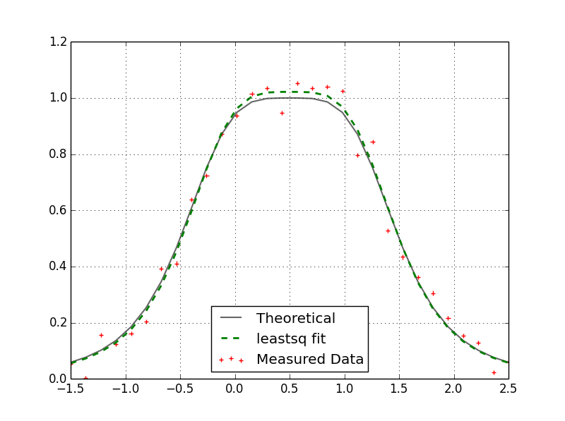
Levenberg-Marquardt algorithm (found here). It's taken me awhile but I finally figured out how to call this routine from Python. There is a Python interface for levmar called PyLevmar but I couldn't get that working. If you have a model written in Python that you are trying to fit to some measured data it is possible to use the C++ levmar routine but not recommended. Most of the routine's time is spent evaluating the function at various points (especially if you do not have an analytical expression for the Jacobian) and if it has to do this in Python you will see a marked slow down. So, while it will cost you some more development time, it is recommended to implement your model in C++ as well. I have taken a simple example here of the Lorentzian function. Suppose we have a bunch of measured values that we want to fit to a function of three parameters (parameter vector p). Our optimization routine should be able to give us the three parameters (p[0], p[1], and [2]) that best fit this data. Here is an example of such a fit:
To this end I created a Python module I can import into Python that will optimize this problem for us. From Python, I wanted to be able to send my initial guess of p, my measured data, and the x-values these measurements were taken at and have returned the parameter values as well as the optimization information. To interface with C++ from Python, I made use of the 
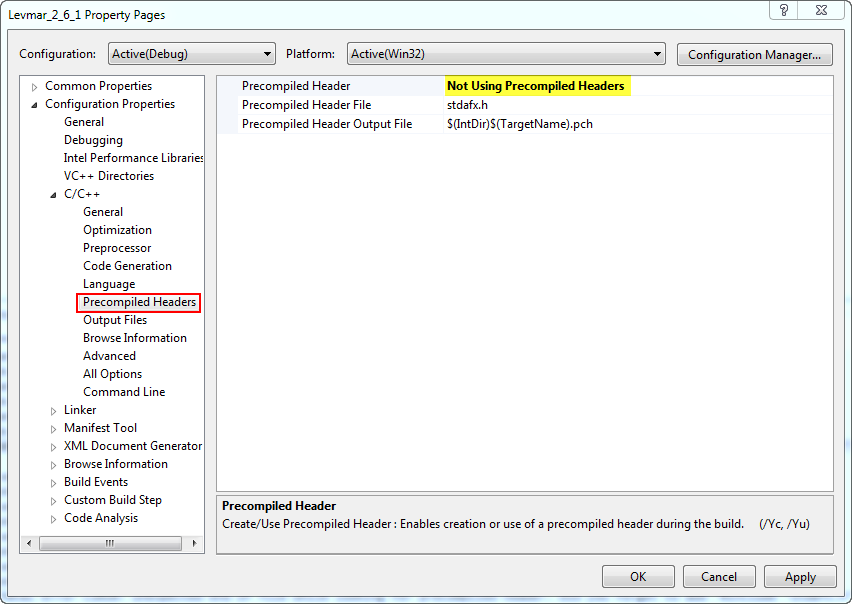
Numpy C-API. You can use Cython for this as well and it would probably be easier to implement but I haven't tried that yet. Using Microsoft's Visual Studio program I created a static library of the levmar routine in a separate project. I then reference that library in this DLL (pyd) module. My C++ code is as follows:

#include "Python.h"
#define NPY_NO_DEPRECATED_API NPY_1_7_API_VERSION
#include "arrayobject.h"
#include <iostream>
#include <iomanip>
#include <cmath>
#include <cfloat>
#include "levmar.h"
using namespace std;

struct argstruct {
 double *xval;
};

double lorentz(double *p, double x) {
 return p[2] / (1.0 + pow((x / p[0] - 1.0), 4) * pow(p[1], 2));
}

void lorentzfit(double *p, double *x, int m, int n, void *data) {
 register int i;
 struct argstruct *xp;
 double xval;
 xp = (struct argstruct *) data;

 for(i=0; i<n i++) {
  xval="xp-">xval[i];
  x[i] = lorentz(p, xval);
 }
}

static PyObject *levmarfit(PyObject *self, PyObject *args) {
 PyArrayObject *xval, *yval, *p0, *results;
 npy_intp *dimx, *dimy, *dimp;
 argstruct adata;
 int ndx, ndy, ndp, ret, parse_ind;
 double *x, *p;
 double opts[LM_OPTS_SZ] = {LM_INIT_MU, 1E-15, 1E-15, 1E-20, -LM_DIFF_DELTA};
 double info[LM_INFO_SZ];

 parse_ind = PyArg_ParseTuple(args, "O!O!O!", &PyArray_Type, &xval, &PyArray_Type, &yval, &PyArray_Type, &p0);
 if (!parse_ind) {
  PyErr_SetString(PyExc_StandardError, "Parsing of function arguments failed. Check function inputs.");
  return NULL;
 } else {
  if (PyArray_TYPE(xval) != NPY_DOUBLE || PyArray_TYPE(yval) != NPY_DOUBLE || PyArray_TYPE(p0) != NPY_DOUBLE) {
   PyErr_SetString(PyExc_TypeError, "Argument inputs are not of type \"double\".");
   return NULL;
  }
 }
 ndx = PyArray_NDIM(xval);
 ndy = PyArray_NDIM(yval);
 ndp = PyArray_NDIM(p0);
 if (ndx != 1 || ndy != 1 || ndp != 1) {
  PyErr_SetString(PyExc_AssertionError, "The dimension of the function input(s) not equal to 1");
  return NULL;
 }
 dimx = PyArray_SHAPE(xval);
 dimy = PyArray_SHAPE(yval);
 dimp = PyArray_SHAPE(p0);
 if (dimx[0] != dimy[0]) {
  PyErr_SetString(PyExc_AssertionError, "The length of x and y vectors are not equal");
  return NULL;
 }
 if (dimp[0] != 3) {
  PyErr_SetString(PyExc_AssertionError, "Length of initial parameter vector not equal to 3.\
              \nThe function being fitted takes 3 parameters.");
  return NULL;
 }
 
 adata.xval = (double *) PyArray_DATA(xval);
 x = (double *) PyArray_DATA(yval);
 p = (double *) PyArray_DATA(p0);

 ret = dlevmar_dif(lorentzfit, p, x, (int)dimp[0], (int)dimy[0], 100000, opts, info, NULL, NULL, (void *) &adata);

 results = (PyArrayObject *) PyArray_SimpleNewFromData(1, dimp, NPY_DOUBLE, (void *) p);
 return Py_BuildValue("(O,[d,d,i,i,i,i])",results, info[0], info[1], (int)info[5], (int)info[6], (int)info[7], (int)info[9]); 
}

static PyMethodDef pylevmarmethods[] = {
 {"levmarfit", levmarfit, METH_VARARGS, "Joel Vroom"},
 {NULL, NULL, 0, NULL}
};

PyMODINIT_FUNC initpylevmar1(void) {
 Py_InitModule("pylevmar1", pylevmarmethods);
 import_array();
}
Granted, it is a lot of code for something you could easily do in Python but, in some cases, you are dealing with complicated models (eg. Heston's semi-analytical option pricing model) that simply take way too long in Python. When this code is compiled, you can use the resultant pylevmar1.pyd file as follows (see lines #3 and #34):
import numpy as np
from scipy.optimize import leastsq
import matplotlib.pyplot as plt
import pylevmar1 
np.random.seed(22)


def lorentz(p,x):
    return p[2] / (1.0 + (x / p[0] - 1.0)**4 * p[1]**2)
   
def errorfunc(p,x,z):
        return lorentz(p,x)-z
   
p = np.array([0.5, 0.25, 1.0], dtype=np.double)
x = np.linspace(-1.5, 2.5, num=30, endpoint=True)
noise = np.random.randn(30) * 0.05
z = lorentz(p,x)
noisyz = z + noise
p0 = np.array([-2.0, -4.0, 6.8], dtype=np.double) #Initial guess

##---------------------------------------------------------------------------##
## Scipy.optimize.leastsq
solp, ier = leastsq(errorfunc, 
                    p0, 
                    args=(x,noisyz),
                    Dfun=None,
                    full_output=False,
                    ftol=1e-15,
                    xtol=1e-15,
                    maxfev=100000,
                    epsfcn=1e-20,
                    factor=0.1)
##---------------------------------------------------------------------------##
## C++ Levmar                       
(sol, info) = pylevmar1.levmarfit(x, noisyz, p0)
##---------------------------------------------------------------------------##

Here I am comparing my C++ levmar result with the scipy.optimize.leastsq result. Both results match and yield:
p = array([ 0.50708339,  0.26618568,  1.02169709])
When I throw these two routine's in a loop and execute them 10,000 times (with different noise) you can see the speed improvement (183x):
Scipy.optimize.leastsq runtime.....263.484s
C++ Levmar runtime........................1.439s

Thursday, August 22, 2013

Sending a Python Function to C++ and Calling Within C++

I thought I would share something I figured out how to do recently. In C++ I have a nice function that numerically integrates a given function. I wanted to be able to call this quadrature routine from Python while feeding it a Python function (callable). For the sake of simplicity I will show a much smaller example here. I realize there are quadrature routines in scipy.integrate but I wanted the flexibility of my C++ routine as well.

Suppose we have a very simply Python function called "myfunc":
def myfunc(x):
    return 2.0 * x;
I want to be able to send this function to C++ and use it within my C++ program. To do this I wrote the following C++ code:
#include "Python.h"

static PyObject *execMyPyFunc(PyObject *self, PyObject *args) {
 PyObject *Fx, *pyresult;
 double x, result;

 PyArg_ParseTuple(args, "dO", &x, &Fx);
 pyresult = PyObject_CallFunction(Fx, "d", x);
 result = PyFloat_AsDouble(pyresult);
 return Py_BuildValue("d", result);
}

static PyMethodDef C_API_TestMethods[] = {
 {"execMyPyFunc", execMyPyFunc, METH_VARARGS, "Add documentation here...."},
 {NULL, NULL}
};

PyMODINIT_FUNC initC_API_Test(void) {
 Py_InitModule("C_API_Test", C_API_TestMethods);
}
This creates a DLL (or .pyd for Python) module called "C_API_Test" that I can import into Python. This module contains the function "execMyPyFunc" that I can use within my Python scripts. The function "execMyPyfunc" takes two arguments:
  1. a double precision scalar
  2. a python function
I make use of PyObject_CallFunction. My Python script looks like this:
from C_API_Test import execMyPyFunc

def myfunc(x):
    return 2.0 * x;
    
fx = execMyPyFunc(1.28,myfunc)
print fx
And it returns 2.56! Voila! Note: I haven't read up on PY_INCREF & Py_DECREF. They may need to be added here. If someone knows, please let me know. Thanks!

Tuesday, August 13, 2013

This is a simple test to incorporate the SyntaxHighlighter in my blog. Quite handy!
import sys, copy
from xml.sax.drivers.drv_xmlproc_val import *
 
class myParser(SAX_XPValParser):
    """XML parser."""
 
    psl = None
 
    def handle_doctype(self, rootname, pub_id, sys_id):
        self.dtd_handler.doctypeDecl(rootname, pub_id, sys_id, self.psl)
 
 
class docHandler:
    """XML Document events handler."""
 
    def characters(self, ch, start, length):
        """Handle a character data event.
        The data are contained in the substring of ch
        starting at position start and of length length."""
 
        print ch[start:start+length],
 
    def endDocument(self):
        """Handle an event for the end of a document."""
I found the instructions here quite helpful!

Monday, July 22, 2013

Tuning the levmar implementation

There are probably many ways to tune the levmar program to the system you are running it on. I highlight three below that I have come across.

On line 54 of the file "misc.h" we have:
#define __BLOCKSZ__ 32 


The properties of the system I am using are shown below via the CPU-Z program.


Given my larger L1 cache I bumped up this value from 32 to 64 (64 * 64 * 8 = 32,768 bytes).

On line 683 of the file "lmbc_core.c" there are seven choices for different linear solvers. I selected the SVD option for its robustness.
issolved=AX_EQ_B_SVD(jacTjac, jacTe, Dp, m); ++nlss; linsolver=AX_EQ_B_SVD;

Friday, July 19, 2013

Building levmar in Visual Studio with Intel's Math Kernel Library (MKL)

Often, when calibrating financial models to market data, we need access to an optimization routine that minimizes the error between theoretical results and actual market results. This allows our model to "fit" the market data as best as possible. And often times the minimization function we are interested in is non-linear. In relatively small problems one can use Matlab's "lsqnonlin" or Python's "scipy.optimize.leastsq" built-in functions. They work quite well but they are slow. I came across this C++ implementation on the internet: levmar. This is a very powerful routine built from the Levenberg-Marquardt optimization algorithm. I was very keen to try this program but faced difficulties compiling it in Microsoft's Visual Studio. The package is very easily compiled in Unix systems where LAPACK is already included. I primarily work in the Windows environment however so I needed a way of building this solution in Visual Studio. In Visual Studio 2008, 2010, and 2012 I have successfully built the executable as follows:

First create a new Visual Studio project (File -> New -> Project).
Select the Win32 Console Application and give your project a name.


I removed the files (stdafx.h, stdafx.cpp, etc.) that came with the new project (I'm not sure if this is necessary or desirable). From the levmar files downloaded from the website I copied all of the C source and header files to my new project folder (excluding everything else):
C:\Users\Joel\Documents\Visual Studio 2012\Projects\Levmar_2_6_1\Levmar_2_6_1\


Once the files are in the project folder, from the Visual Studio Solution Explorer I right click on "Source Files" and select Add -> Existing Item. But we only add the C files that don't end in "_core". 
From the README file:
Notice that *_core.c files are not to be compiled directly; For example,
Axb_core.c is included by Axb.c, to provide single and double precision
routine versions.
 Similarly, we add the header files to the "Header Files" folder in the Solution Explorer.


Now, if you try to build this project, you will probably be greeted with the following error message:
fatal error C1010: unexpected end of file while looking for precompiled header. Did you forget to add '#include "stdafx.h"' to your source?
To get around this I selected the following:


If we try to build our project with this change we will see the following errors:
Build started: Project: Levmar_2_6_1, Configuration: Debug Win32 ------
1>Build started 19/07/2013 2:06:05 PM.
1>InitializeBuildStatus:
1>  Touching "Debug\Levmar_2_6_1.unsuccessfulbuild".
1>ClCompile:
1>  All outputs are up-to-date.
1>  misc.c
1>  lmlec.c
1>  lmdemo.c
1>  lmbleic.c
1>  lmblec.c
1>  lmbc.c
1>  lm.c
1>  Axb.c
1>  Generating Code...
1>Axb.obj : error LNK2019: unresolved external symbol _dgeqrf_ referenced in function _dAx_eq_b_QR
1>Axb.obj : error LNK2019: unresolved external symbol _dorgqr_ referenced in function _dAx_eq_b_QR
1>lmlec.obj : error LNK2001: unresolved external symbol _dorgqr_
1>Axb.obj : error LNK2019: unresolved external symbol _dtrtrs_ referenced in function _dAx_eq_b_QR
1>Axb.obj : error LNK2019: unresolved external symbol _dpotrf_ referenced in function _dAx_eq_b_Chol
 
1>misc.obj : error LNK2019: unresolved external symbol _dgemm_ referenced in function _dlevmar_trans_mat_mat_mult
1>misc.obj : error LNK2019: unresolved external symbol _dpotf2_ referenced in function _dlevmar_chol
1>c:\users\joel\documents\visual studio 2012\Projects\Levmar_2_6_1\Debug\Levmar_2_6_1.exe : fatal error LNK1120: 30 unresolved externals
1>
1>Build FAILED.
1>
1>Time Elapsed 00:00:01.24
========== Build: 0 succeeded, 1 failed, 0 up-to-date, 0 skipped ==========
And the reason for this is that the build process cannot link to the LAPACK libraries (not included inWindows). Apparently there are ways to add this to Windows but I was unsuccessful in my endeavors. What I did instead was download a trial version of Intel's "Composer XE 2013" program. Even though this program will expire after the trial period ends we're not actually interested in the program. Rather, we are interested in the library files that get installed (as far as I know, these do not expire). If you install this program in the default directory you will see this folder:
C:\Program Files (x86)\Intel\Composer XE 2013\mkl\lib\ia32
which contains the math kernel we are interested in. To link our Visual Studio project to these libraries, do the following:


and add the following dependency:


Now we will be able to successfully build our project. The resultant executable file will be found in your project's folder (either Debug or Release depending on what you have selected). From the command prompt, I can run the executable and see the following results:


Which are just the results of the selected optimization problem found in the lmdemo.c file. It worked!

Eventually I would like to modify this project to create a library that I can call from other programs. I may also try to create a DLL out of this that I can call from Python.